
| Citation: |
Dan-yi Su, Bin-bin Guo, Qian-yong Liang, Chu-jin Liang, Fei-long Lin, Su-meng Jiang, Yi-fei Dong, Xue-min Wu, 2023. Application of the monitoring and early warning system for internal solitary waves: Take the second natural gas hydrates production test in the South China Sea as an example, China Geology, 6, 676-684. doi: 10.31035/cg2022043

|
Application of the monitoring and early warning system for internal solitary waves: Take the second natural gas hydrates production test in the South China Sea as an example
-
Abstract
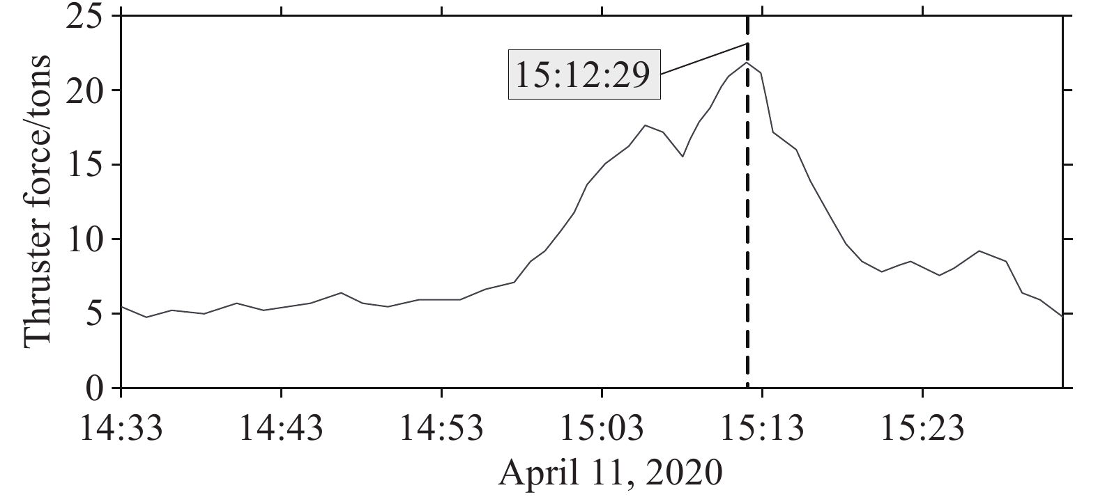
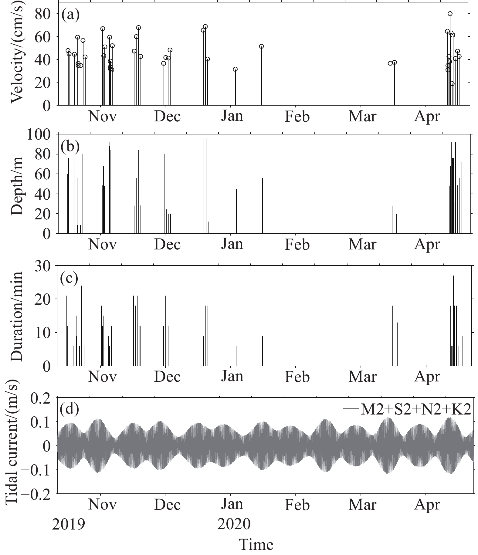
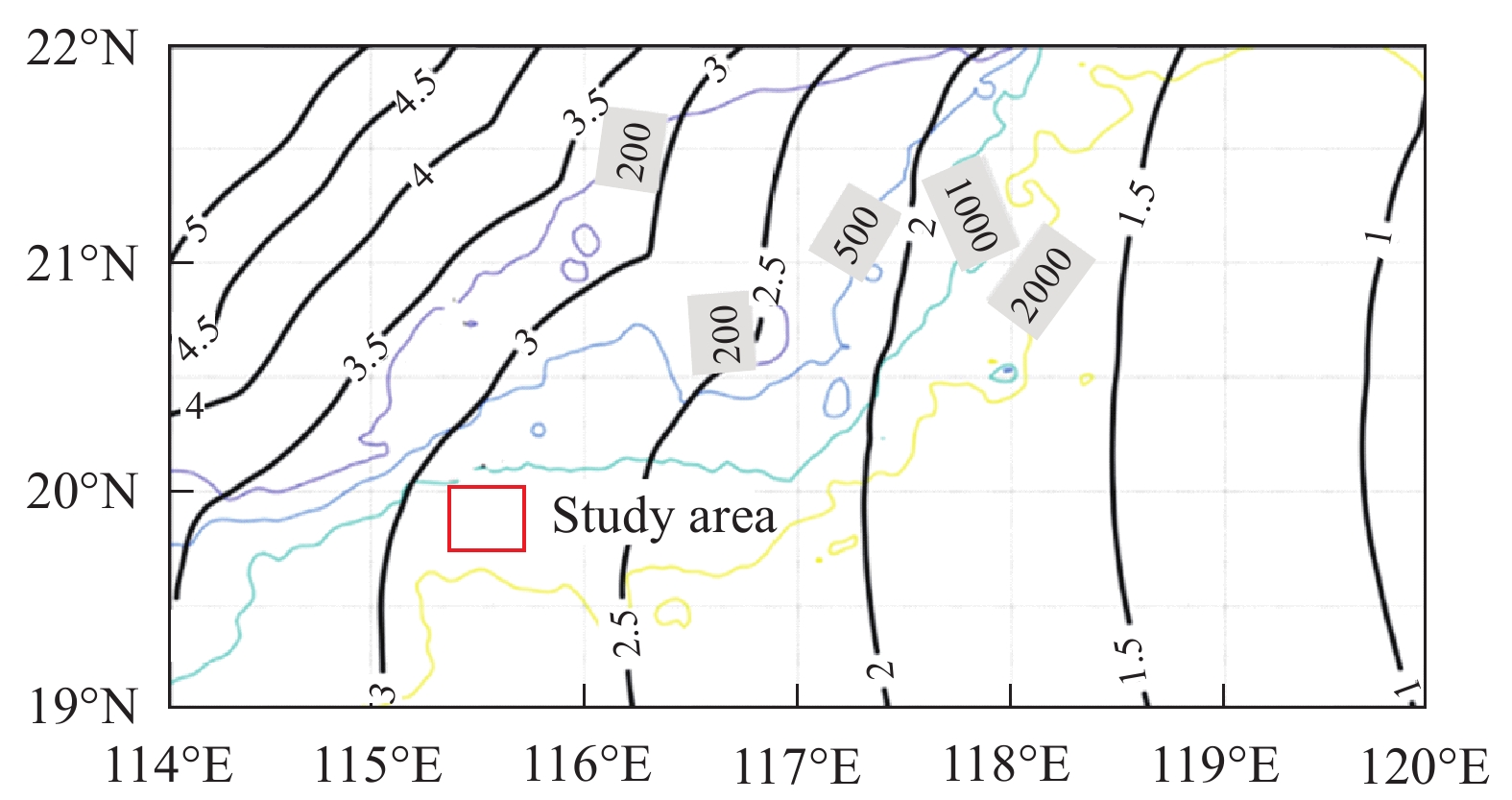
Internal solitary waves (ISWs) contain great energy and have the characteristics of emergency and concealment. To avoid their damage to offshore engineering, a new generation of monitoring and early warning system for ISWs was developed using technologies of double buoys monitoring, intelligent real-time data transmission, and automatic software identification. The system was applied to the second natural gas hydrates (NGHs) production test in the Shenhu Area, South China Sea (SCS) and successfully provided the early warning of ISWs for 173 days (from October 2019 to April 2020). The abrupt changes in the thrust force of the drilling platform under the attack of ISWs were consistent with the early warning information, proving the reliability of this system. A total of 93 ISWs were detected around the drilling platform. Most of them occurred during the spring tides in October–December 2019 and April 2020, while few of them occurred in winter. As suggested by the theoretical model, the full-depth structure of ISWs was a typical current profile of mode-1, and the velocities of wave-induced currents can reach 80 cm/s and 30 cm/s, respectively, in the upper ocean and near the seabed. The ISWs may be primarily generated from the interactions between the topography and semidiurnal tides in the Luzon Strait, and then propagate westward to the drilling platform. This study could serve as an important reference for the early warning of ISWs for offshore engineering construction in the future.
-

-
References
Buijsman MC, Kanarska Y, McWilliams JC. 2010. On the generation and evolution of nonlinear internal waves in the South China Sea. Journal of Geophysical Research: Oceans, 115(C2). doi: 10.1029/2009jc005275. Cai SX, Huang QZ, Qiu Z, Mai BQ. 2000. A numerical study on dynamic mechanism of internal tide. Tropic Oceanology, 19(3), 27–32 (in Chinese). Cai SQ, Xie JS, He JL. 2012. An Overview of internal solitary waves in the South China Sea. Surveys in Geophysics, 33(5), 927–943. doi: 10.1007/s10712-012-9176-0. Cai SQ, et al. 2015. Numerical model of internal isolated wave and its application in the South China Sea. Beijing. China Ocean Press. 1–158 (in Chinese). Chen L, Zheng QA, Xiong XJ, Yuan YL, Xie HR, Guo YL, Yu L, Yun SJ. 2019. Dynamic and statistical features of internal solitary waves on the continental slope in the northern South China Sea derived from mooring observations. Journal of Geophysical Research: Oceans, 124, 4078–4097. doi: 10.1029/2018jc014843. Chun MH, Leng XD, Liang SS, Wang Z, Luo XQ, Yang XD, Xu S. 2021. Research and application of internal wave monitoring and warning technology in South China Sea. Petroleum Engineering Construction, 47(4), 70–74 (in Chinese). Du T, Tseng YH, Yan XH. 2008. Impacts of tidal currents and Kuroshio intrusion on the generation of nonlinear internal waves in Luzon Strait. Journal of Geophysical Research:Atmospheres, 113, C08015. doi: 10.1029/2007jc004294. Duda TF, Lynch JF, Irish JD, Beardsley RC, Ramp SR, Chiu CS, Tang TY, Yang YJ. 2004. Internal tide and nonlinear internal wave behavior at the continental slope in the Northern South China Sea. IEEE Journal of Oceanic Engineering, 29(4), 1105–1130. doi: 10.1109/joe.2004.836998. Ebbesmeyer CC, Coomes CA, Hamiton RC. 1991. New observations on internal waves (solitons) in the South China Sea using an acoustic doppler current profiler. Marine Technology Society Journal, 91, 165–175. Egbert GD, Bennett AF, Foreman MGG. 1994. TOPEX/POSEIDON tides estimated using a global inverse model. Journal of Geophysical Research: Atmospheres, 99(C12), 24821–24852. doi: 10.1029/94jc01894. Egbert GD, Erofeeva SY. 2002. Efficient inverse modeling of barotropic ocean tides. Journal of Atmospheric and Oceanic Technology, 19(2), 183–204. doi: 10.1175/1520-0426(2002)0192.0.CO;2. Fang XH, Du T. 2005. Fundamentals of Oceanic Internal Waves and Internal Waves in the China Seas. China Qingdao, Ocean University of China Press, 337 (in Chinese). Gerkema T. 2001. Internal and interfacial tides: beam scattering and local generation of solitary waves. Journal of Marine Research, 59, 227–255. doi: 10.1357/002224001762882646. Goff M, Jeans G, and Harrington-Missin L, Baschenis C. 2010. Soliton early warning system for offshore applications. Oceanology International (OI), London, United Kingdom. Grimshaw R, 1985. Evolution equations for weakly nonlinear long internal waves in a rotating fluid. Stud. Studies in Applied Mathematics, 73(1), 1–33. doi: 10.1002/sapm19857311. He JX, Zhong CM, Yao YJ, Yan P, Wang YL, Wan ZF, Guan J, Zhang JF. The exploration and production test of gas hydrate and its research progress and exploration prospect in the northern South China Sea. Marine Geology Frontiers, 2020, 36(12): 1-14. doi: 10.16028/j.1009-2722.2020.127 (in Chinese). Holloway PE, Pelinovsky E, Talipova T, Barnes B. 1997. A nonlinear model of internal tide transformation on the Australian North West Shelf. Journal of Physical Oceanography, 27(6), 871–896. doi: 10.1175/1520-0485(1997)027<0871:ANMOIT>2.0.CO;2. Hsu MK, Liu AK, Liu C. 2000. A study of internal waves in the China Seas and Yellow Sea using SAR. Continental Shelf Research, 20(4-5), 389–410. doi: 10.1016/s0278-4343(99)00078-3. Huang XD, Chen ZH, Zhao W, Zhang ZW, Zhou C, Yang QX, Tian JW. 2016. An extreme internal solitary wave event observed in the northern South China Sea. Scientific Reports, 6(1), 30041. doi: 10.1038/srep30041. Hu WJ, Liu ZL, Chen B. 2015. Impacts of internal waves in the South China Sea on deepwater drilling safety and corresponding countermeasures. Oil Drilling & Production Technology, 37(1), 160–162 (in Chinese). Jackson CR. 2009. An empirical model for estimating the geographic location of nonlinear internal solitary waves. Journal of Atmospheric and Oceanic Technology. 26(10), 2243–2255. doi: 10.1175/2009jtecho638.1. Joseph RI, Egri R. 1978. Multi-soliton solutions in a finite depth fluid. Journal of Physics A:Mathematical and General, 11(5), 97–102. doi: 10.1088/0305-4470/11/5/002. Lee CY, Beardsley RC. 1974. The generation of long nonlinear internal waves in a weakly stratified shear flow. Journal of Geophysical Research: Atmospheres, 79(3), 453–462. doi: 10.1029/jc079i003p00453. Li MJ. 2012. Three-dimensional Numerical Simulation and Analysis of Internal Tides in the Northern South China Sea. Beijing, University of Chinese Academy of Sciences, Ph. D thesis, 1–116 (in Chinese). Li Q, Farmer DM. 2011. The generation and evolution of nonlinear internal waves in the deep basin of the South China Sea. Journal of Physical Oceanography, 41(7), 1345–1363. doi: 10.1175/2011jpo4587.1. Liu AK, Hsu MK, Liang NK. 1998. Evolution of nonlinear internal waves in China Seas, Journal of Geophysical Research: Atmospheres, 103 (C4), 7995–8008. Liu AK, Ramp SR, Zhao YH, Tang TY. 2004. A case study of internal solitary wave propagation during ASIAEX 2001. IEEE Journal of Oceanic Engineering, 29(4), 1144–1156. doi: 10.1109/joe.2004.841392. Maxworthy T. 1979. A note on the internal solitary waves produced by tidal flow over a three-dimensional ridge. Journal of Geophysical Research:Atmospheres, 84(C1), 338. doi: 10.1029/jc084ic01p00338. Pierini S. 1989. A model for the Alboran Sea internal solitary wave. Journal of Physical Oceanography, 19, 755–772. doi: 10.1175/1520-0485(1989)019<0755:AMFTAS>2.0.CO;2. Ramp SR, Tang TY, Duda TF, Lynch JF, Liu AK, Chiu CS, Bahr FL, Kim HR, Yang YJ. 2004. Internal solitons in the northeastern South China Sea Part I: sources and deep water propagation. Journal of Oceanic Engineering, 29(4), 1157–1181. doi: 10.1109/JOE.2004.840839. VanGastel P, Ivey GN, Meuleners MJ, Antenucci JP, Fringer O. 2009. The variability of the large-amplitude internal wave field on the Australian North West Shelf. Continental Shelf Research, 29(11–12), 1373–1383. doi: 10.1016/j.csr.2009.02.006. Wang HP, Chen L, Guo YL, Cao LZ, Hu XM, Xiong XJ. 2021. Observing, identification and early warning technology of internal solitary wave and its application in Liuhua 16-2 oilfield group development project. The Ocean Engineering, 39(2), 162–170 (in Chinese). Xiong LL, Yang CP, Wu JQ, Gao HF, Yao YJ, Li XJ, Zhu XY, Cheng ZH. 2020. Characteristics of stratigraphic sedimentary in the south-north continental margin basin of the South China Sea and its differential control on hydrocarbon accumulation. Geology in China, 47(5), 1407–1425. doi: 10.12029/gc20200508. Yang YJ, Fang YC, Chang MH, Ramp SR, Kao CC, Tang TY. 2009. Observations of second baroclinic mode internal solitary waves on the continental slope of the northern South China Sea. Journal of Geophysical Research:Oceans, 114, C10003. doi: 10.1029/2009jc005318. Ye JL, Qin XW, Xie WW, Lu HL, Ma BJ, Qiu HJ, Liang JQ, Lu LA, Kuang ZG, Lu C, Liang QY, Wei SP, Yu YJ, Liu CS, Li B, Shen KX, Shi HX, Lu QP, Li J, Kou BB, Song G, Li B, Zhang HE, Lu HF, Ma C, Dong YF, Bian H. 2020. The second natural gas hydrate production test in the South China Sea. China Geology, 3(2), 197–209. doi: 10.31035/cg2020043. You YX, Hu TQ, Xu H, Yu Z, Fang YL, Shi ZM, Qu Y, Xiao Y. 2010. Experiments on interaction of internal waves with semi-submersible platform in a stratified fluid. Chinese Journal of Theoretical and Applied Mechanics, 42(3), 400–406 (in Chinese). Zhang Z, Fringer OB, Ramp SR. 2011. Three-dimensional, nonhydrostatic numerical simulation of nonlinear internal wave generation and propagation in the South China Sea. Journal of Geophysical Research:Oceans, 116, C05022. doi: 10.1029/2010jc006424. Zhao Z, Klemas V, Zheng Q, Yan XH. 2004. Remote sensing evidence for baroclinic tide origin of internal solitary waves in the northeastern South China Sea. Geophysical Research Letters, 31(6), L06302. doi: 10.1029/2003gl019077. Zhao JR, Xie B, Su J, Wang SS, Li B. 2018. Transient mooring analysis of a semi-submersible drilling platform under internal wave condition. Ship Science and Technology, 40(21), 75–79 (in Chinese). -
Access History
Figures(10)
Tables(3)

Export File
Citation
Dan-yi Su, Bin-bin Guo, Qian-yong Liang, Chu-jin Liang, Fei-long Lin, Su-meng Jiang, Yi-fei Dong, Xue-min Wu, 2023. Application of the monitoring and early warning system for internal solitary waves: Take the second natural gas hydrates production test in the South China Sea as an example, China Geology, 6, 676-684. doi: 10.31035/cg2022043
Format
Content
 DownLoad:


-
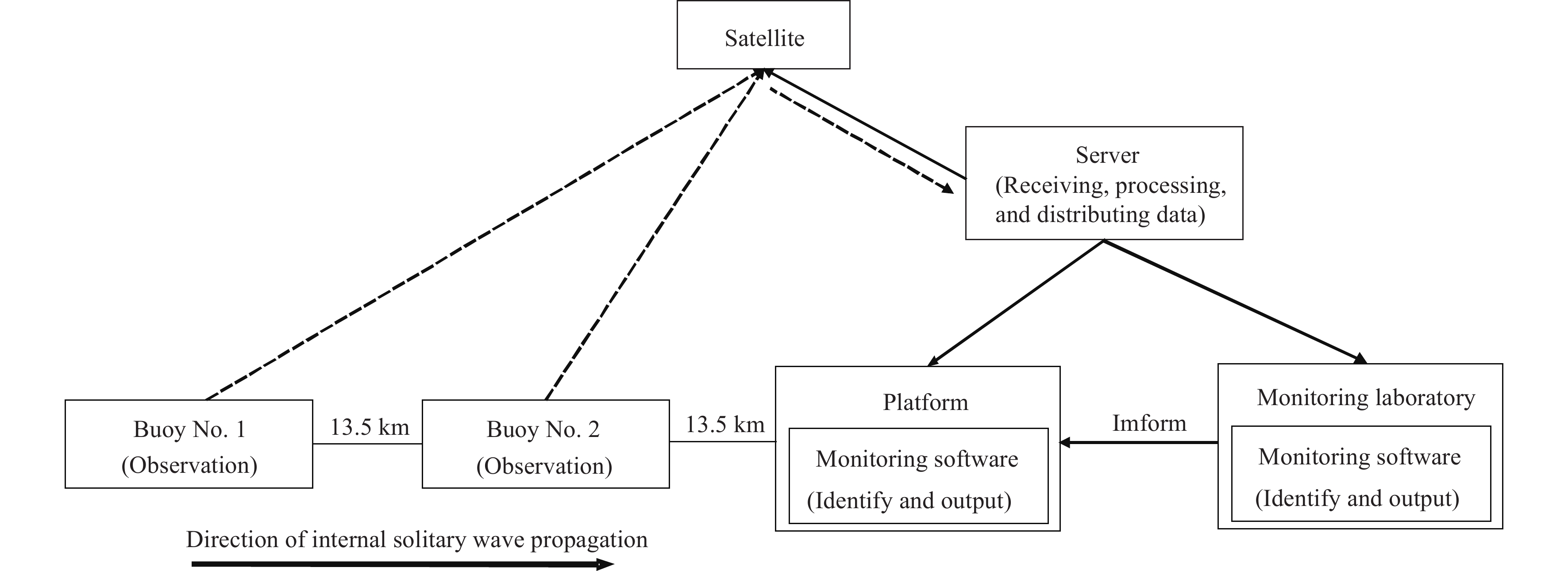
Figure 1.
Technical framework of the monitoring and early warning system for ISWs.
-
Figure 2.
Locations of the drilling platform and monitoring buoys in the second NGHs production test. The red box denotes the study area (i.e., the target area for the monitoring and early warning of ISWs); the yellow box denotes the site of tide forecast data; the red triangles indicate the buoy stations; the black square is the position of the drilling platform; and the black lines indicate the water depth (unit: m).
-
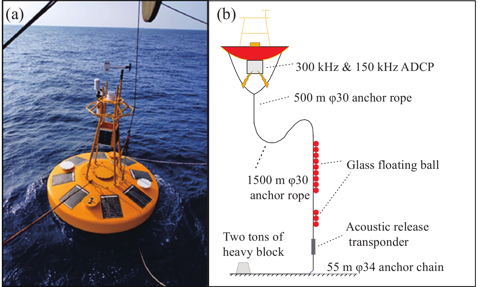
Figure 3.
Structure of a buoy used in the ISW System. Physical picture (a); overall structure (b).
-
Figure 4.
Velocity profiles of upper ocean currents (a, b) and average velocity at 0–100 m (c, d) when the strongest ISW passed through buoys No. 2 (left) and No. 1 (right) on April 11, 2020.
-
Figure 5.
Changes in the thrust force of the drilling platform when the strongest ISW passed on April 11, 2020 (unit: tons).
-
Figure 6.
Time series of ISWs in the study area. Velocity of wave-induced currents (a); depth of the maximum velocity (b); duration of the ISWs (c); semidiurnal tides near the Luzon Strait (d).
-
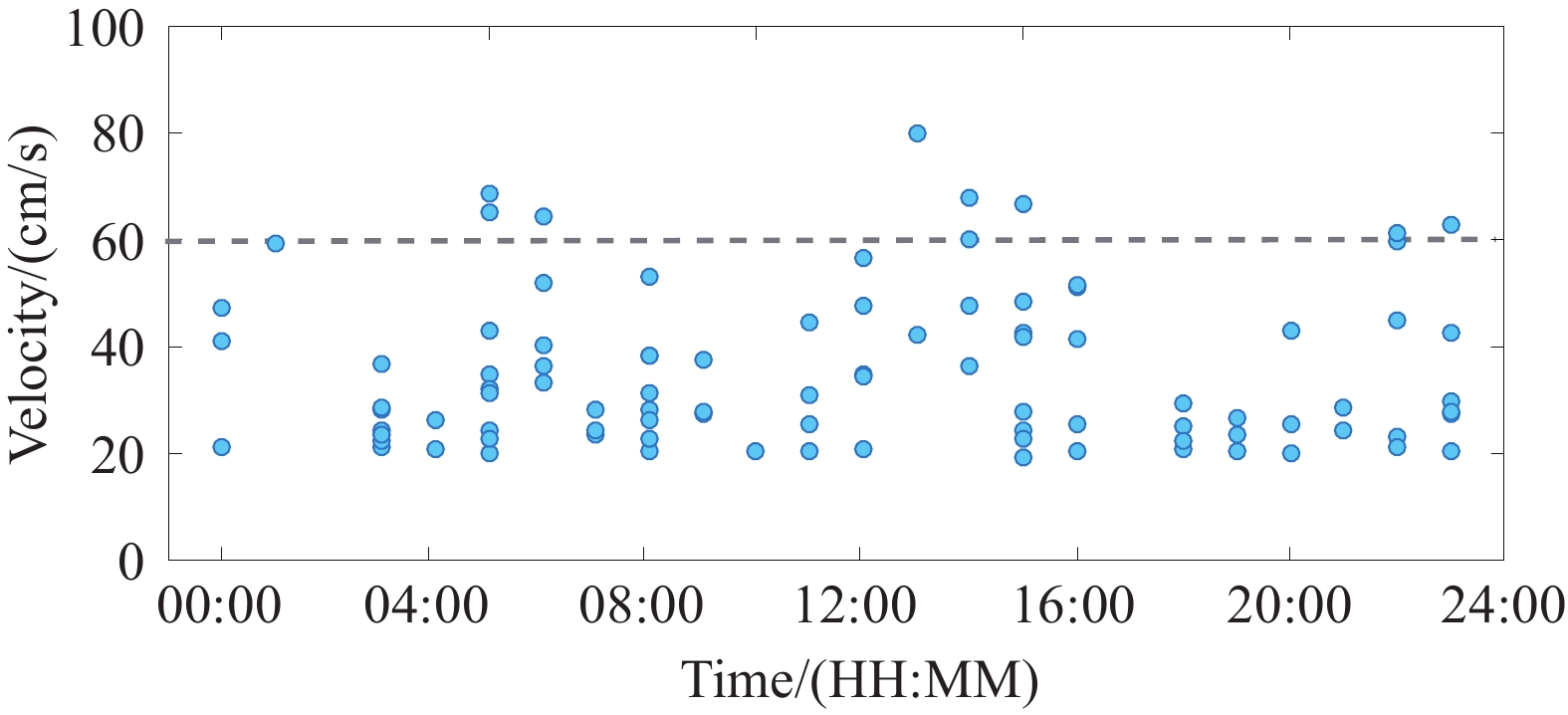
Figure 7.
Daily distribution of the velocity of wave-induced currents during the monitoring.
-
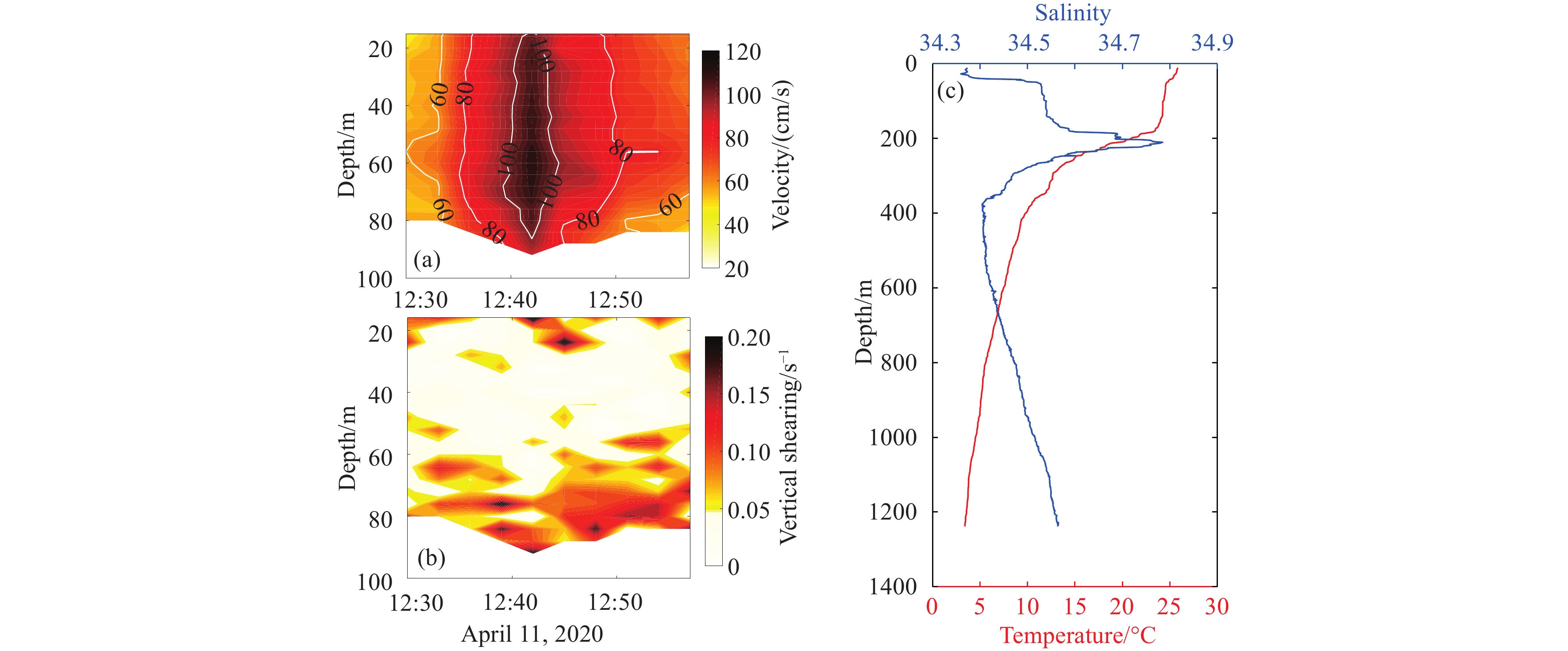
Figure 8.
The horizontal velocity profile (a) and the vertical shear profile (b) when the strongest ISW passed by buoy No. 2 on April 11, 2020, and the temperature vs. salinity profile (c) near buoy No. 2 in April 2021.
-
Figure 9.
Vertical structure of the strongest ISW passed by buoy No. 2 on April 11, 2020. Simulation results at 0‒100 m (a); monitoring results at 0‒100 m (b); simulated full-depth structure (c).
-
Figure 10.
Time it takes for ISWs to propagate from the Luzon Strait to the study area (black solid lines; unit: day). The colorful solid lines denote water depth (unit: m), and the red box denotes the study area.